


Degeneracy and Sampling on a Rectangular Grid
Created on October 18 at 12:12 pm - by: admin
This post is the second part of a multiple part series covering triangulation and interpolation using Igor Pro 7.
- Part 1: Planar Triangulations
- Part 2: Degeneracy and Sampling on a Rectangular Grid
- Part 3: Triangulation on the Surface of a Sphere and Triangulations in 3D
- Part 4: 3D Interpolation
In the previous blog post I reviewed linear and Voronoi interpolations of scatter data. In this blog post I focus on the more common case where data are sampled on a regular rectangular grid.
I'll start with the simplest example where an arbitrary set of scalars {zi} sampled at the vertices of the rectangle ABCD. The simplest surface connecting the set of points {zi} can be constructed by dividing the rectangle into two triangles. The two possible ways to triangulate the rectangle are shown in Figure 1.
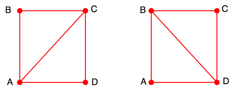
Figure 1: The two possible triangulations for a rectangle ABCD.
To illustrate the difference between the two triangulations consider interpolated values inside the rectangle. For this example I chose the following z-values for the points ABCD: {1, 2, 1.5, 1}. Figure 2 shows interpolated values inside the rectangle. The interpolation inside each triangle is based on the z-values at its vertices.
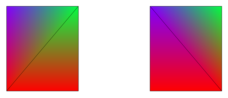
Figure 2: Interpolated values displayed using Rainbow256 colormap.
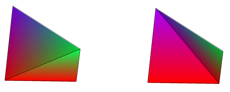
Figure 3: Side view of the two surfaces clearly shows how different they are despite the fact that they have identical vertex values.
The state of the two possible triangulations is described as degeneracy. It is formally defined as a condition where a set of 4 or more co-circular sampling sites have a circle passing through them that does not contain any other sampling site in its interior.
As I mentioned in the introduction, this issue is fairly common because it is present whenever you sample on a rectangular grid. In most cases it is easy to ignore because the sampling is sufficiently dense. The motivation for this blog post is to illustrate what happens when the sampling is not dense.
An image plot representing the four values we used above is shown in Figure 4.
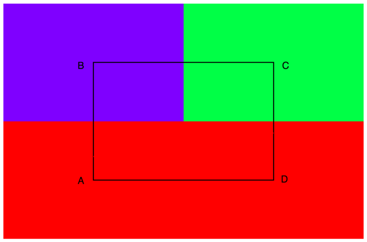
Figure 4: Four large pixels of the values {1, 2, 1.5, 1}
Now suppose you wanted to add a contour representing the value 1.2. Depending on the choice of triangulation you might have slightly different contours as shown in Figure 5.
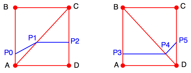
Figure 5: Two contour traces for the value 1.2 shown in blue. The exterior intersection points {p0, p3} and {p2, p5} respectively are identical.
Since there is no obvious solution to the degeneracy problem, Igor's triangulation algorithm (ImageInterpolate with the keyword Voronoi) introduces a slight random perturbation in the XY locations so that four vertices are not likely to remain co-circular in the XY plane. Although this approach should work in general, it is still better to avoid triangulating data sampled on a rectangular grid.
Igor's standard contour algorithm applied to this data produces the contour in Figure 6. In this case the trace consists of a single line segment from one edge of the rectangle to the other. Although this algorithm appears to solve the triangulation degeneracy we discussed above, it is subject to a different type of degeneracy.
The algorithm for computing contour lines for data sampled on a rectangular grid produces a contour by combining the line segments drawn between the points at which the desired contour level intersects the edges of the rectangle. For the ABCD rectangle there are two intersection points with the 1.2 level: one on the AB side and the other on the CD side. In this case there is no ambiguity in drawing the contour line.
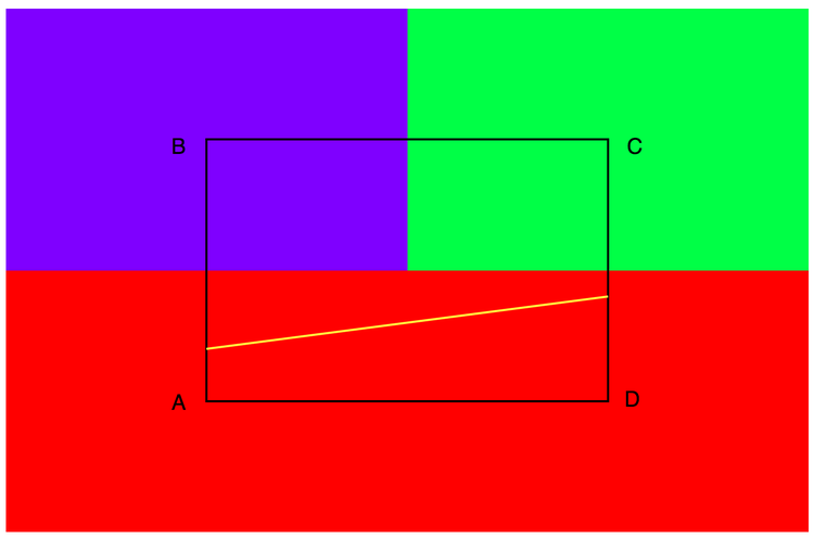
Figure 6: A contour trace for the value 1.2 (yellow).
Now suppose the values at the ABCD vertices are: {1, 2, 1, 2} respectively, and suppose the contour level remains at 1.2 (see Figure 7). In this case we have an intersection of the contour level with each edge of the rectangle. Recalling that contour lines must either close on themselves or close on the boundary of the domain, we have the following contour choices:
1. P0-P3 and P1-P2.
2. P0-P1 and P2-P3.
3. P0-P1-P2-P3-P0.
The last choice is valid only if ABCD is also the boundary of the data. To see why that is the case, consider the next data rectangle BCEF for example. This rectangle must have at least two intersections with the 1.2 level and so the contour P2-P1 would have to continue into the BCEF instead of closing towards P0 or stopping at P1.
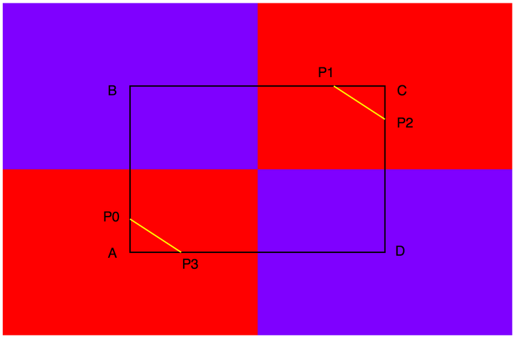
Figure 7: A contour trace for the value 1.2 (yellow).
Igor's contour algorithm chooses to connect P0-P3 and P1-P2. This is equivalent to using the diagonal BD for triangulation. If the triangulation used the diagonal AC then the resulting contour consists of the segments P0-P1 and P2-P3.
In most applications there is no need to worry about these details unless you are interested in sub-pixel resolution or if you are working with a very small data set. If your data are sampled on a rectangular grid you should not need to triangulate it; the triangulation is automatic and is outside user control.

Forum

Support

Gallery
Igor Pro 9
Learn More
Igor XOP Toolkit
Learn More
Igor NIDAQ Tools MX
Learn More